
|
Book Home Page Bloglines 1906 CelebrateStadium 2006 OfficeZealot Scobleizer TechRepublic AskWoody SpyJournal Computers Software Microsoft Windows Excel FrontPage PowerPoint Outlook Word Host your Web site with PureHost! |
Monday, March 01, 2010 – Permalink – Video TutorialsWhat you see"MIStupid.com is The Online Knowledge Magazine that publishes information that everyone should know, wants to know, or forgot.A few of the lessons include:
See all Topics excel Labels: Tutorials <Doug Klippert@ 3:42 AM
Comments:
Post a Comment
Tuesday, February 02, 2010 – Permalink – Office TrainingSuggestionsTechRepublic lists a number of areas that you might explore when training is needed for a new Office version.Here are a few:
See all Topics excel Labels: Tutorials <Doug Klippert@ 3:55 AM
Comments:
Post a Comment
Tuesday, December 22, 2009 – Permalink – Link WorkbooksTie them togetherExcel is a flatfile database, but you can do some Access kinds of relationships. "A link is a formula that gets data from a cell in another workbook. When you open a workbook that contains links (a linking workbook), Microsoft Excel reads in the latest data from the source workbook or workbooks (updates the links).
See all Topics excel <Doug Klippert@ 3:10 AM
Comments:
Post a Comment
Tuesday, November 24, 2009 – Permalink – Formatting OverviewLooking goodThe judicious use of formatting can make data easier to understand as well as pleasant to see. Scott Lowe put together a series of articles on how to format data in Excel. The Articles are on TechRepublic.com Anatomy of Excel formatting: Part 1
See all Topics excel <Doug Klippert@ 3:39 AM
Comments:
Post a Comment
Thursday, October 29, 2009 – Permalink – Hep MeHelp topic locationsThis from Ron de Bruin:
Help Context IDs for Excel See all Topics excel <Doug Klippert@ 3:09 AM
Comments:
Post a Comment
Sunday, October 11, 2009 – Permalink – Update Excel on the WebAuto RepublishYou can save an Excel file as a Web page and makes it easy to update data in a worksheet that has already been saved to the Web. Here is how to save an Excel file as a Web page and set it up it for automatic updates:
Save Excel as Web Page DevX.com: Four Ways to Use Excel on the Web Penn State: Interactive Excel on the Web See all Topics excel <Doug Klippert@ 3:49 AM
Comments:
Post a Comment
Thursday, September 17, 2009 – Permalink – Lock the BarnProtect your workJohn Walkenbach has put together an FAQ on Workbook/Worksheet/VBA protection. Spreadsheet Protection FAQ The Microsoft Knowledge Base article KB 293445 Has a list of references to protection information. Here is more information Overview of security and protection in Excel See all Topics excel <Doug Klippert@ 3:44 AM
Comments:
You might want to check out Mike Alexander's blog post about how easy it is to remove worksheet protection in Excel 2007.
Post a Comment
http://datapigtechnologies.com/blog/index.php/hack-into-a-protected-excel-2007-sheet/
Friday, September 11, 2009 – Permalink – AutoShapesDrawing bar objectsKim Hedrich has put together a series of basic articles on AutoShapes for TechTrax. AutoShapesPart 1 - How to draw circles, ovals, squares and rectangles; also modifying fill and line colour AutoShapes Part 2 - Fill Effects AutoShapes Part 3 - Shadows and 3-D AutoShapes - Text Inside a Shape See all Topics excel <Doug Klippert@ 3:13 AM
Comments:
Post a Comment
Saturday, August 22, 2009 – Permalink – Self HelpGet started in the right directionThe Office of Technology Services of Towson University, located in Towson, Md., provides Self-Help Training Documents for many applications. They are available for many levels of knowledge. They’re clean, clear, and concise.
See all Topics excel Labels: Tutorials <Doug Klippert@ 3:06 AM
Comments:
Post a Comment
Thursday, July 16, 2009 – Permalink – Access-Excel-XML-HTMLTransfer dataXML makes data transferable between applications. Here is a tutorial with downloadable files. Some simple guidance of how to transfer data from Excel or Access into HTML web pages using XML data files. VBA programs can be used to export data tables from Excel or Access into simple XML files. There are several examples of using different methods to display the XML and XSL files on web pages in order to quickly share your data with others. An introduction to Excel and XML data files Also: Some nice photos and calendar layout: Monthly calendar with photos See all Topics excel <Doug Klippert@ 3:56 AM
Comments:
Post a Comment
Tuesday, June 30, 2009 – Permalink – Thirtieth Condition FormattingThree is not always enoughPre-2007 Excel gives the user the ability to specify up to three conditions under Format>Conditional Formatting. If that is not enough, Frank Kabel and Bob Phillips of xlDynamic.com offer a free download that extends the conditions to 30!  Extended Conditional Formatter Also see: Conditional Formatting (including 2007) See all Topics excel <Doug Klippert@ 3:09 AM
Comments:
Post a Comment
Thursday, April 09, 2009 – Permalink – Excel-lent E-MailOutlook, Excel, and VBARon de Bruin, Microsoft MVP - Excel, has put together a collection of VBA routines to make Excel e-mail friendly. See if these topics tempt you: Example Code for sending mail from Excel
Also see: <Doug Klippert@ 3:27 AM
Comments:
Post a Comment
Sunday, March 22, 2009 – Permalink – Intro to ExcelEnglish ExcelThe UCL (University College London) site for the High Energy Physics Group of the Department of Physics & Astronomy, has an introduction to Excel e-book on this page. It's the material used in a 10 week course. "This web page contains material for the computing and data analysis elements of the first-year PHYS1B40 Practical Skills course. Here are some links to the topics covered topics: Excel Data Analysis Visual Basic See all Topics excel Labels: Tutorials <Doug Klippert@ 3:35 AM
Comments:
Post a Comment
Friday, March 13, 2009 – Permalink – Web QueriesDo You Question the Web?This feature can make data acquisition a lot easier than Copy-Paste-Reformat-Try again. "Generally, though, people tend to overlook the option of using the Web as a data source for Excel, be that source the Internet, an intranet, an extranet, or a Web Service. But they shouldn't. Web queries are an easy, yet remarkably flexible and predictable way of bringing data into Microsoft Excel from anywhere on the Web. You can point a Web query at any HTML document that resides on any Web server - or even on a file server, for that matter - and pull part or all of the contents back into your spreadsheet...When you start using Excel's Web queries, you will realize they are almost as limitless as the Web is. Well Kept Secret On the menu bar, go to Data>Import External Data. (In 2007, Data>Get Extrnal Data>From Web). Then, select Import Data to use an existing Web query or select New Web Query to build a new one.  Also see: Vertex42.com: Excel Web Query Secrets Revealed MSDN.Microsoft.com/library Integrate Far-Flung Data into Your Spreadsheets with the Help of Web Services Updating Excel From the Web And: Web Queries and Dynamic Chart Data in Excel 2002 See all Topics excel <Doug Klippert@ 3:49 AM
Comments:
Post a Comment
Wednesday, February 25, 2009 – Permalink – Hide DigitsSimple obfuscationThe kid said, "Daddy, I know the secret password! It's star, star, star, star!" **** You can use functions to hide parts of sensitive data. Social Security Number 555-55-5555 =CONCATENATE("***-**-", RIGHT(B2,4)) Combines the last four digits of the SSN with the "***-**-" text string (***-**-5555)  Credit Card Number 5555-5555-5555-5555 =CONCATENATE(REPT("****-",3), RIGHT(B3,4)) Repeats the "****-" text string three times and combines the result with the last four digits of the credit card number (****-****-****-5555) Microsoft Office Online: Display only the last four digits of identification numbers See all Topics excel <Doug Klippert@ 3:14 AM
Comments:
Post a Comment
Wednesday, January 14, 2009 – Permalink – Spreadsheet DesignMake it work and look goodTimothy Miller uses the nom de screen of "Jethro" (Moses' Father-in-Law). His SpyJournal.biz site/blog gives some tips on how to present an Excel solution
You'll find the complete text here: Design Presentation Tips Also see: SpreadsheetStyle See all Topics excel <Doug Klippert@ 3:02 AM
Comments:
Post a Comment
Sunday, December 14, 2008 – Permalink – Format NumbersIt's your choiceHere is an almost forgotten sample spreadsheet. It was constructed, for Microsoft, back in 1997 by Lori B. Turner, and is still relevant. The sheets are protected. In order to see the cell formatting, you need to go to Tools>Protection to Unprotect Sheet . . . There is no password required Formatting sample Workbook Also: OzGrid:
You still owe the sum of 5,434 for invoice # 2232 from 6/15/2001
<Doug Klippert@ 3:14 AM
Comments:
Post a Comment
Sunday, November 23, 2008 – Permalink – Array FormulasGood orderly directionAn array is defined as "An orderly arrangement". It can be thought of as a collection of data packaged in a container. The individual items in the container can be selected by referring to their location; first, second, and so on.
"Have you ever sat in front of your monitor pulling your hair out trying to identify duplicate entries in a list? If so, you should learn about Microsoft Excel's array formulas. In fact, you can use array formulas to perform calculations that are otherwise impossible in Excel, and you can enhance the power of some of the program's existing functions." Excel's Array Formulas By Helen Bradley Chip Pearson: Introduction To Array Formulas "Array Formulas are formulas that work with arrays, instead of individual numbers, as arguments to the functions that make up the formula"
<Doug Klippert@ 3:33 AM
Comments:
Post a Comment
Saturday, November 15, 2008 – Permalink – Locate Duplicates with Conditional FormattingHighlight entriesConditional formatting can be set up by selecting the whole range, or for the first cell in the range and then copy down that conditional format. I find it is usually just as easy to select the whole range to start with. The formula will adjust itself. In this example, cell B2 has a heading of Product Numbers. Select cell B3 (or the entire targeted range) and from the menu. Select Format > Conditional Formatting. The Conditional Formatting dialog opens with the initial dropdown saying "Cell Value Is". Click the arrow next to this, and choose "Formula Is". After selecting "Formula Is", the dialog box changes appearance. Instead of boxes for "Between x and y", there is now a single formula box. You can type in any formula as long as that formula will evaluate to TRUE or FALSE. The formula to type in the box is =COUNTIF(B:B,B3)>1 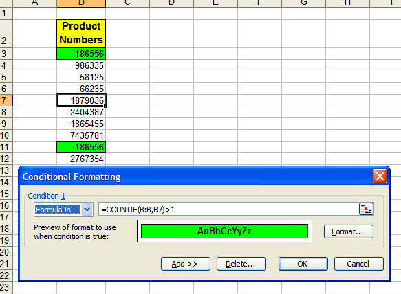 This says, "look through the entire range of column B. Count how many cells in that range are the same value as what is in B3." (In the graphic, B7 is the Active cell.) That same comparison will be made in every cell that contains the conditional formatting. (If your data is in column E and you are setting the first conditional formatting up in E5, the formula would be =COUNTIF(E:E,E5)>1.) Anytime a duplicate appears in the range, it will receive the special formatting. In this example, any time a duplicate number appears anywhere in column B, even if it is not itself formatted, the selected range will reflect the duplicate. =COUNT(B:B,B3)>2 would count entries that appear more than two times. =COUNT(B:B,B3)=2 would count entries that appear twice. If you want only a part of the column in the formula, it is easier to use absolute addresses, such as =COUNT($B$3:$B$200,B3)>1 Adapted from MrExcel.com Also see: Chip Pearson's discussion of duplicates: Contextures.com: Conditional Formatting (See Hide Duplicate Values) See all Topics excel <Doug Klippert@ 3:45 AM
Comments:
Post a Comment
Saturday, November 01, 2008 – Permalink – What if?Scenario suggestions"I wonder how our net profit would be affected if we could reduce our variable cost per unit by just a few cents. How much could we save if we found a lower interest rate? Wouldn't it be nice to be able to play around with some scenarios, do some "what-ifs" — without messing up your current data? It's easy with Microsoft Office Excel . You can set up "scenarios" to experiment with the data and compare the possibilities. Who knows? It could be a road map to better solutions for your business." Excel "what-if" scenarios American Institute of Certified Public Accountants (AICPA.org): " To find out how to use what-if functions, follow along as this tutorial takes you step-by-step through several problems. Excel 2000 is used here to illustrate these concepts, but the process is similar in all spreadsheet programs." Using a spreadsheet to do "what-if" analyses <Doug Klippert@ 2:29 AM
Comments:
Post a Comment
Wednesday, October 15, 2008 – Permalink – Download DemonstrationsStill good after all these yearsBack in the day, Barnes Consulting was a major player with Office 97. They've gone on to other consulting areas, but you can still study what they called "On-Line Experiences".
Downloadable Learning Experiences See all Topics excel <Doug Klippert@ 3:21 AM
Comments:
Post a Comment
Wednesday, October 01, 2008 – Permalink – Data ComparisonNo formulasThe Data Consolidation technique allows you to compare lists quickly and easily. With the Consolidation technique, you can identify the number of duplicate entries in two or more lists without using a formula. (not that it's easier, just that there are no formulas)
 The numbers appears in Column B are the totals of the list number in Column B. If the result = 1, the name appears in List 1 and does not appear in List 2. If the result = 2, the name appears in List 2 and does not appear in List 1. If the result = 3, the name appears in both lists (1+2=3). The action is not dynamic, so if you make changes, the Consolidation must be rerun. From: "Mr Excel ON EXCEL" (Holy Macro Books) Also see: John Walkenbach: Comparing Two Lists With Conditional Formatting Chip Pearson: Duplicate And Unique Items In Lists Here's a more complex method: Microsoft Office Online: Use Excel to compare two lists of data Also: BetterSolutions.com: What are Consolidated Worksheets ? See all Topics excel <Doug Klippert@ 4:16 AM
Comments:
Post a Comment
Tuesday, September 30, 2008 – Permalink – Access Data - Excel Time SheetsDistribute to everyoneMany times an office will provide Excel for all users, but not want or need to also install Access on every desk. Helen Feddema has laid out a method to use the data in an Access database to create Excel workbooks. These workbooks can then be e-mailed to employees to be used to record time spent on projects. The code provided is above the entry level user, but understandable. There is a downloadable file that includes the instructions and samples of the Access and Excel files. Go to Access Archon Columns from Woody's Office Watch.
<Doug Klippert@ 3:17 AM
Comments:
Post a Comment
Sunday, September 28, 2008 – Permalink – Video TutorialsFree instructionsMichael Alexander has produced a collection of about 60 online video demonstrations of some interesting Excel maneuvers.
All About Pivot Tables
All About Charts
 And More: DataPig Technologies See all Topics excel Labels: Tutorials <Doug Klippert@ 5:01 AM
Comments:
Post a Comment
Wednesday, September 24, 2008 – Permalink – Statistics and ExcelWhat are the chances"Excel is the widely used statistical package, which serves as a tool to understand statistical concepts and computation to check your hand-worked calculation in solving your homework problems. The site provides an introduction to understand the basics of and working with the Excel. Redoing the illustrated numerical examples in this site will help improving your familiarity and as a result increase the effectiveness and efficiency of your process in statistics."
The site is very clearly written. While some of the concepts are advanced, Dr. Arsham explains them in simple terms. It is a good introduction to the Analysis ToolPak.
The University of Baltimore: Statistical Data Analysis See all Topics excel Labels: Tutorials <Doug Klippert@ 4:30 AM
Comments:
Post a Comment
Thursday, September 18, 2008 – Permalink – Excel Charts For DummiesGraph-ologyYou don't have to be spreadsheet challenged to read this book. Many people become quite adept at using Worksheet functions and even VBA, but have little experience with charting. This book has some great cartoons, and, by page 361, the reader will be exposed to step by step instructions covering both simple charts and some quite sophisticated graphing. "Excel Charts For Dummies will show readers how to professionally display data in presentation-quality charts. How to create attractive charts and why to use specific charts in particular circumstances. Lots of real-world examples with step-by-step tutorials. How to embed graphics and pictures into charts; then use them in impressive PowerPoint presentations or Microsoft Word documents. The book features a 16-page full-color insert of the best Excel charts 'works of art.'" Ken Bluttman is also the author of Excel Formulas and Functions for Dummies, Access Hacks, and Developing Microsoft Office Solutions. By Ken Bluttman ISBN 0-7645-8473-1 Wiley Publishing, Inc. 2005 Technical editor Doug Klippert See all Topics excel <Doug Klippert@ 6:40 AM
Comments:
Post a Comment
Thursday, September 04, 2008 – Permalink – Running Total in CommentCircular solutionYou can't have a worksheet formula that looks like this: =C3+C3 But you can do something similar if you use VBA and store the results in another location. "In Microsoft Excel you can avoid circular references when you create a running total by storing the result in a non-calculating part of a worksheet. This article contains a sample Microsoft Visual Basic for Applications procedure that does this by storing a running total in a cell comment."
<Doug Klippert@ 12:06 PM
Comments:
Post a Comment
Monday, July 14, 2008 – Permalink – Column(s) FunctionVLOOKUP"Excel will adjust cell references in formulas when you insert or delete rows or columns.
Also: <Doug Klippert@ 5:25 AM
Comments:
Post a Comment
Tuesday, June 10, 2008 – Permalink – Auto LinkOutlook Contacts in AccessAutomatically set up links to data outside of Access. It still works in Access/Outlook '07. Try this:
 The changes made in Access will be reflected in Outlook and vice versa. If you want to create a new database that will link to other data that isn't in an Access format, you can do it quickly. The classic way is to use the File>Get External Data >Link Tables method. However you can simply choose File >Open from the menu bar. Select the appropriate data format from the Files Of Type dropdown list (such as Microsoft Excel (*.xls)). Open the file and Access will automatically create an MDB file with the same name as the data source you selected and will set up links to the data. From there you can develop forms, queries and reports. See all Topics See all Topics excel <Doug Klippert@ 7:54 AM
Comments:
Post a Comment
Thursday, May 29, 2008 – Permalink – Fill HandleDouble click the handleIf you have a column of data, you may wish to insert a new formula on each row, number the lines, or add a date column. To fill the column down to the bottom of the database, just double-click on the fill handle - the tiny square at the bottom right corner of the active cell. The duplication continues as long as there are entries in the adjacent column. If you wish to fill down a series, make at least two entries so that the interval is apparent. For instance if there is a column of data in A1:A400, enter the number "1" in B1, "2" in B2. Select B1:B2. Double click on the fill handle and Excel will fill the series down to B400. You can also select a longer series, such as the name of a supervisor and the team members. Format the supervisors name differently, if you want. Select the list and double click the fill handle. The list will be repeated down the page, as long as there is a corresponding entry in an adjacent column. The formatting will also be repeated. Also: Custom Lists
Click Options on the Tools menu and click the Edit tab. (Use the Office button in the upper left corner in 2007) <Doug Klippert@ 6:20 AM
Comments:
Post a Comment
Saturday, May 17, 2008 – Permalink – Enter in Multiple WorkSheetsGroup sheetsA common use for Excel is to keep periodic statistics; sales by quarter, or phone calls per month. It can be tedious to try to create worksheets for each month and include duplicate data such as client or salesperson's names. Set up the workbook with as many worksheets that may be needed; perhaps one for each month and one for cumulative year-end totals. Click the tab for the first month, hold down the SHIFT key and select the last worksheet in the series. All the sheets are now chosen. You will see [Group] on the Title bar. Enter any common information on the first sheet and it will be duplicated on all of the grouped sheets. When you are done, Right-click a sheet tab and choose Ungroup Sheets on the context menu. Non-contiguous sheets can be selected using the Ctrl key. If the sheets are grouped, they will all be printed together. Also:
<Doug Klippert@ 7:51 AM
Comments:
Post a Comment
Sunday, May 04, 2008 – Permalink – Conditional FormattingIf it's Tuesday, it must be mauve
This can be very useful for highlighting important information and values outside an accepted range or providing a visual cue to associate value ranges with color codes. Just click the cells you'd like to format and select Format >Conditional Formatting. The Conditional Formatting dialog box lets you set up the conditions by which the formatting of the cell will occur. You pick the operator (between, equal to, less than, etc.) and the value or range of values. Click Format to open the Format Cells dialog box, where you can select the colors and styles to be used. However, you can format that same cell to exhibit red, bolded text on a green background if it contains a value between 51 and 100. GR Business Process Solutions: Also <Doug Klippert@ 7:03 AM
Comments:
Post a Comment
Tuesday, April 08, 2008 – Permalink – Date and Time EntryMonth Day, Day MonthQDE An Excel Date Entry Add-In Ron de Bruin "QDE is a fully-functional Excel Add-in that provides quick input of dates, in all international formats. It handles quick data entry interpretation and reflects the three interacting issues of Date System, Day, Month Year ordering, and number of digits used in the quick date entry. With QDE you enter just as many digits as needed to clearly identify the date, QDE will do the rest."
<Doug Klippert@ 6:18 AM
Comments:
Post a Comment
Thursday, March 13, 2008 – Permalink – Accustom Yourself to ExcelShake hands with a worksheetAnneliese Wirth has written an article for Office.Microsoft.com about how to get used to the new user interface in Excel 2007.
Surviving the switch to Excel 2007 See all Topics excel <Doug Klippert@ 7:20 AM
Comments:
Post a Comment
Saturday, March 01, 2008 – Permalink – OLAP CubesMore dimensions than Star trek
<Doug Klippert@ 7:09 AM
Comments:
Post a Comment
Tuesday, January 29, 2008 – Permalink – Split the CostsSplit the sheets (?)Joe Chirilov presents a spreadsheet solution to a friendship breaker. Recently a large group of friends and I went on a multi-city tour of Europe that lasted a couple weeks. There was a lot of planning that went into this trip and responsibilities for booking different legs of the trip were spread out across the group. How do you efficiently handle paying back multiple people while getting reimbursed for your costs at the same time? You can download the spreadsheet here:Split_Costs.zip <Doug Klippert@ 6:53 AM
Comments:
Post a Comment
Monday, December 10, 2007 – Permalink – Chiropractics for ExcelHEADINGKnead and pound numbers Chad Rothschiller, a program manager on the Excel team, discusses using formulas to 'clean up' data in Excel. Excel is a great tool to use when you need to take data in one format, manipulate it into another format, and push the results along to another process, e.g. a database. In this context, Excel is a great landing pad or middle man, serving as a data transformation tool to move data from one system to another. I'm sure you've been faced with at least one of theses problems:
Manipulate and massage See all Topics excel <Doug Klippert@ 4:50 AM
Comments:
Post a Comment
Monday, November 12, 2007 – Permalink – All the BasicsAll(most) all you need to knowOffice.Microsoft.com has a short demo that shows you the main things anyone needs to know about Excel. There are many thousands of users who find that this is all they ever need.
Use simple formulas to do the math See all Topics excel <Doug Klippert@ 8:00 AM
Comments:
Post a Comment
Thursday, November 01, 2007 – Permalink – Loan PaymentBasic tutorialMicrosoft provides a number of learning activities related to fundamental tasks. Here's one that walks the student through a worksheet designed to calculate interest and total payment for a purchase, based on different loan terms. "This practical spreadsheet lesson offers easy answers to life's perplexing math problems like How much will my dream car really cost after financing? Also: <Doug Klippert@ 5:55 AM
Comments:
Post a Comment
|


